Example usage

So, you’ve generated your design and run your experiements. Now comes the hard part of building the model. So to use doenut in a project you will need some data to fit. We label these inputs and responses. First, let’s load the packages and set the logging level to something appropriate.

import doenut
import pandas as pd
import matplotlib.pyplot as plt

doenut.set_log_level('WARNING')

Now load the responses into dataframes. In this case, we’ve already split the data into two csv files so it is nice and straightforward.

inputs = pd.read_csv("data/inputs.csv")
responses = pd.read_csv("data/responses.csv")['Profit']

inputs

	P	Temp.	Flow	Purge	Cool
0	200.0	300.0	10800.0	0.0	-150.0
1	950.0	300.0	10800.0	0.0	-30.0
2	200.0	600.0	10800.0	0.0	-30.0
3	950.0	600.0	10800.0	0.0	-150.0
4	200.0	300.0	16800.0	0.0	-30.0
5	950.0	300.0	16800.0	0.0	-150.0
6	200.0	600.0	16800.0	0.0	-150.0
7	950.0	600.0	16800.0	0.0	-30.0
8	200.0	300.0	10800.0	25.0	-150.0
9	950.0	300.0	10800.0	25.0	-30.0
10	200.0	600.0	10800.0	25.0	-30.0
11	950.0	600.0	10800.0	25.0	-150.0
12	200.0	300.0	16800.0	25.0	-30.0
13	950.0	300.0	16800.0	25.0	-150.0
14	200.0	600.0	16800.0	25.0	-150.0
15	950.0	600.0	16800.0	25.0	-30.0
16	600.0	450.0	13800.0	15.0	-90.0

responses

0     10901.0
1    -12000.0
2     -5222.0
3     22675.0
4    -12000.0
5     54224.0
6     -3558.0
7     -6188.0
8      5264.0
9    -12000.0
10    -6395.0
11    14140.0
12   -12000.0
13    37206.0
14    -5727.0
15    -7225.0
16    25032.0
Name: Profit, dtype: float64

First, let’s create a fully populated model and see how good that is (or isn’t).

dataset = doenut.data.ModifiableDataSet(inputs, responses)
basic_scaled_model, basic_unscaled_model = doenut.models.AveragedModel.tune_model(dataset)
print(f"Model results: R2 {round(basic_scaled_model.r2, 2)}, Q2 {round(basic_scaled_model.q2, 2)}")

Model results: R2 0.64, Q2 0.18

Well, the R2 is OK, but that is not a good Q2. Let’s try a saturated model. First we need to generate the dataset and build fresh models.

saturated_inputs, saturated_source_list = doenut.add_higher_order_terms(inputs)
saturated_columns = list(saturated_inputs.columns)
print(saturated_columns)
saturated_dataset = doenut.data.ModifiableDataSet(saturated_inputs, responses)
saturated_scaled_model, saturated_unscaled_model = doenut.models.AveragedModel.tune_model(saturated_dataset)
print(f"Model results: R2 {round(saturated_scaled_model.r2, 2)}, Q2 {round(saturated_scaled_model.q2, 2)}")

['P', 'Temp.', 'Flow', 'Purge', 'Cool', 'P**2', 'Temp.**2', 'Flow**2', 'Purge**2', 'Cool**2', 'P*Temp.', 'P*Flow', 'P*Purge', 'P*Cool', 'Temp.*Flow', 'Temp.*Purge', 'Temp.*Cool', 'Flow*Purge', 'Flow*Cool', 'Purge*Cool']
Model results: R2 0.99, Q2 0.76

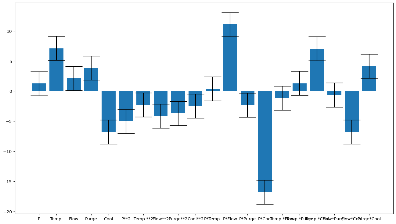
Note that off the bat that is significantly better, but we can still improve. Let’s plot the coefficents to see if any are insignificant. Note that this is what we use the scaled model for - it allows us to compare the coefficients directly.

doenut.plot.coeff_plot(saturated_scaled_model.coeffs, labels=saturated_columns, errors='p95', normalise=True)

Input_selector was: [0, 1, 2, 3, 4, 5, 6, 7, 8, 9, 10, 11, 12, 13, 14, 15, 16, 17, 18, 19]
Average coefficients are: [  1.25306962   7.11379047   2.11312542   3.82547541  -6.78594611
  -5.01631432  -2.27660597  -4.1607204   -3.69115095  -2.50497266
   0.36882115  11.07279902  -2.32877925 -16.79564447  -1.19514006
   1.28809486   7.06118971  -0.64517142  -6.8157383    4.11896796]
Errors are [2. 2. 2. 2. 2. 2. 2. 2. 2. 2. 2. 2. 2. 2. 2. 2. 2. 2. 2. 2.]
Coefficient labels are: ['P', 'Temp.', 'Flow', 'Purge', 'Cool', 'P**2', 'Temp.**2', 'Flow**2', 'Purge**2', 'Cool**2', 'P*Temp.', 'P*Flow', 'P*Purge', 'P*Cool', 'Temp.*Flow', 'Temp.*Purge', 'Temp.*Cool', 'Flow*Purge', 'Flow*Cool', 'Purge*Cool']

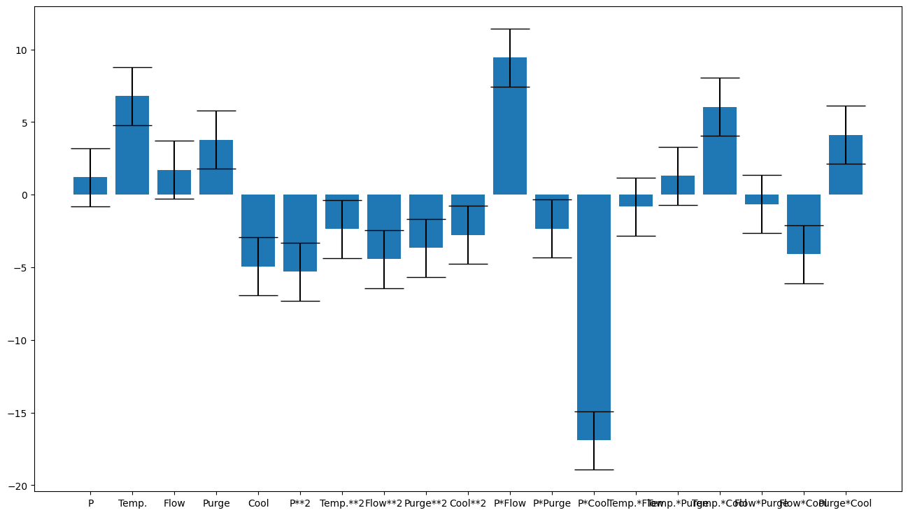
Let’s remove the term P*Temp. To do this, make a list of the columns you want (either names or by column index) and create a filtered version of the dataset

column_selector = [x for x in saturated_columns if x != 'P*Temp.']
filtered_dataset = doenut.data.ModifiableDataSet(saturated_inputs, responses).filter(column_selector)
filtered_scaled_model, filtered_unscaled_model = doenut.models.AveragedModel.tune_model(filtered_dataset)
doenut.plot.coeff_plot(filtered_scaled_model.coeffs, labels=column_selector, errors='p95', normalise=True)
print(f"Model results: R2 {round(filtered_scaled_model.r2, 2)}, Q2 {round(filtered_scaled_model.q2, 2)}")

Input_selector was: [0, 1, 2, 3, 4, 5, 6, 7, 8, 9, 10, 11, 12, 13, 14, 15, 16, 17, 18]
Average coefficients are: [  1.19066062   6.8002752    1.69896309   3.78976886  -4.9481041
  -5.29855244  -2.35390278  -4.42824778  -3.67289423  -2.77328902
   9.43719155  -2.32877925 -16.91237789  -0.81836908   1.28809486
   6.03553243  -0.64517142  -4.0941079    4.11896796]
Errors are [2. 2. 2. 2. 2. 2. 2. 2. 2. 2. 2. 2. 2. 2. 2. 2. 2. 2. 2.]
Coefficient labels are: ['P', 'Temp.', 'Flow', 'Purge', 'Cool', 'P**2', 'Temp.**2', 'Flow**2', 'Purge**2', 'Cool**2', 'P*Flow', 'P*Purge', 'P*Cool', 'Temp.*Flow', 'Temp.*Purge', 'Temp.*Cool', 'Flow*Purge', 'Flow*Cool', 'Purge*Cool']
Model results: R2 0.99, Q2 0.77

A slight improvement in Q2 and we are using fewer terms (generally a good thing). We can also plot how good the fit looks like this:

doenut.plot.plot_observed_vs_predicted(responses, filtered_unscaled_model.predictions)

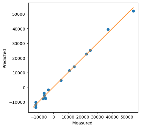
Not bad. Now normally you would continue around the loop a few times, removing terms until you have a nicely parsimonious model, but for the sake of brevity let’s pretend this is the best one (it’s not bad, but there are certainly better ones (Excercise for the reader: You can get a Q2 of 0.862 with this approach - see if you can find it!).